In this tutorial, I cover:
1. What occupancy models are useful for
2. Fitting single-season occupancy models with the R package `unmarked`
3. Testing goodness-of-fit for single-season occupancy models

The code (and sample data) from this tutorial are available on GitHub.

Let's get started!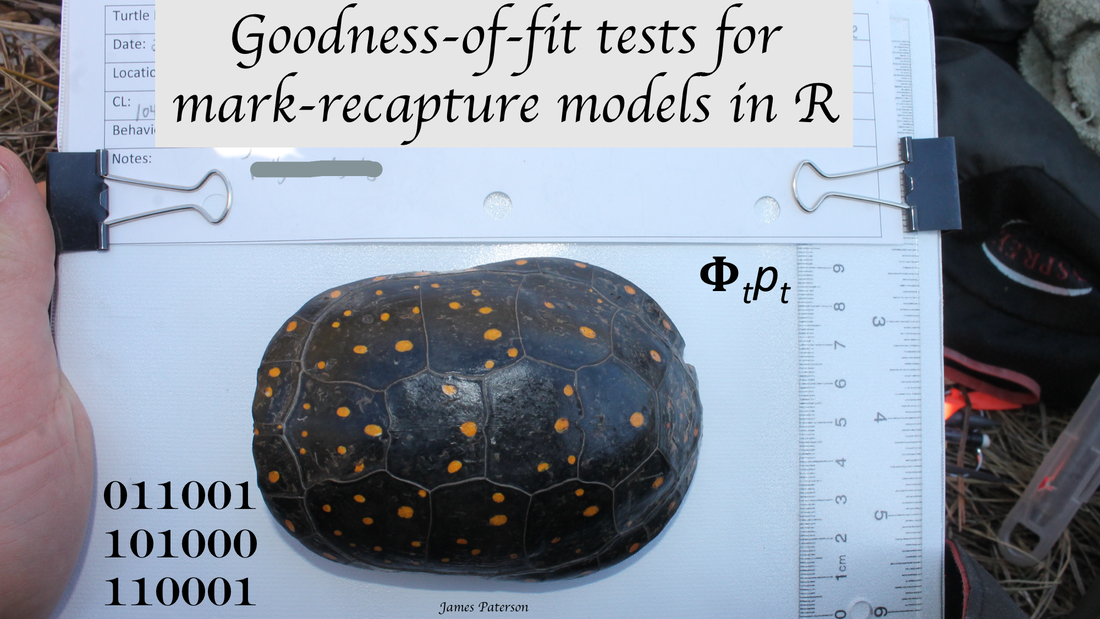

Mark-recapture models are a useful framework to test hypotheses about what drives differences in wildlife survival and detection probability. However, it is important to assess the goodness-of-fit (GOF) for these models before we make inferences.

​What causes lack of fit?

• assumption violations (more on that below!),
• model misspecification (e.g. missing important variables), or
• unmodelled heterogeneity (e.g. some ‘trap happy’ or ‘trap-shy’ animals)

In this tutorial, I cover testing assumptions of the Cormack-Jolly-Seber model using `R2ucare`.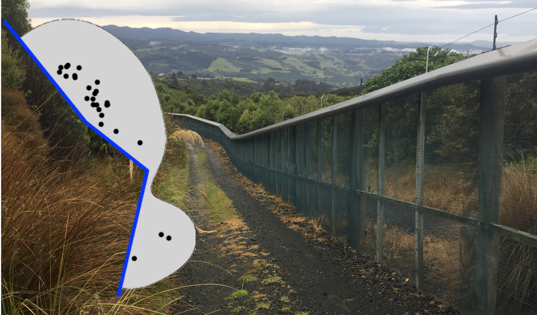

Kernel density estimators are commonly used for estimating the home range of animals (see my previous post on estimating home ranges with kernels).

​But, a common issue is that the kernel contour for an animal extends beyond a boundary the animal cannot cross.

Can we adjust the density estimator and limit kernel contours to not cross boundaries?
The code and data I use in this tutorial are available on my on my GitHub repo.

One of my favourite ways to visualize wildlife tracking data is to animate paths. Using `ggmap` and `gganimate`, it has never been easier to show-off your hard-earned tracking data with animated maps you can use in presentations, meetings, and at dinner parties.

The code and data I use in this tutorial are available on my on my GitHub repo.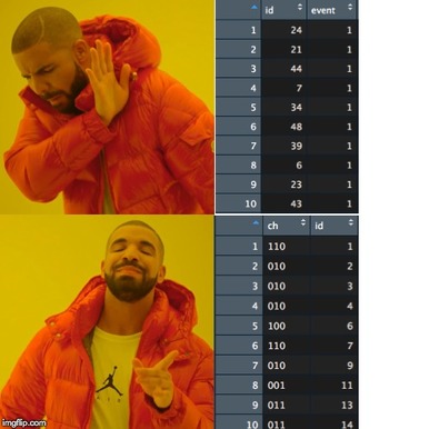

​Do you do mark-recapture analyses? The required input data are "capture histories": binary strings to describe when animals (or plants) were found in a study. 

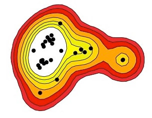
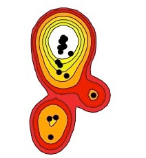
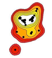
For example, a capture history of "101" describes a study where an individual was:

* caught on the first event, 
* not observed on the second event, and
* observed on the third event.

Data from mark-recapture and mark-resight studies are not usually recorded or stored in this format. Let's run through an exercise to reshape this data into capture histories!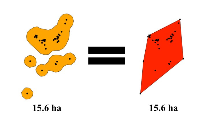

Kernel density estimators are often used for measuring home ranges and this is useful for measuring interactions between animals and their environment. However, kernels are sensitive to the choice of a smoothing factor (h).

For reptiles, Row & Blouin-Demers (2006) recommended using an h that creates a 95% contour area equal to the 100% minimum convex polygon. I have written two functions in R to do this for any tracking data set.

This post will be helpful if you:

• Tracked reptiles (or another animal with a low number of relocations) and are quantifying habitat use,
  
• Want to make your 95% kernel area equal to the 100% minimum convex polygon for each individual.

What is a home range?

"that area traversed by the animal during its normal activities of food gathering, mating and caring for young. Occasional sallies outside the area, perhaps exploratory in nature, should not be considered as in part of the home range.” -Burt 1943
  
The most commonly cited definition is vague and does not provide a clear method for estimating the home range. So what should someone wanting to calculate home ranges do?

The following is adapted from a workshop I ran at Trent University in January 2018. It is meant to be an introduction to using R to analyze movement patterns and home ranges from telemetry data. I have split the content into several smaller posts. In this first post, I format simulated telemetry data for spatial analyses and map points and paths overtop of Google Earth imagery with the ggmap package.

Code available at my GitHub page.